Refinement Strategies for High-Quality Mesh Generation

Introduction

This document explains the importance of mesh refinement in numerical simulation, emphasizing how targeted resolution allocation enhances accuracy and stability. It discusses the pitfalls of uniform refinement, which can lead to unnecessary computational costs, and highlights the value of optimizing mesh element size only where needed. The introduction covers foundational principles, describes how refinement supports predictive and efficient simulations, and introduces different strategies for distributing resolution to address geometric and physical complexities.

mesh_refinement

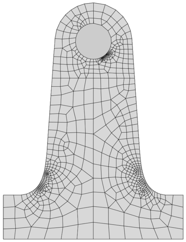
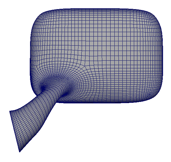
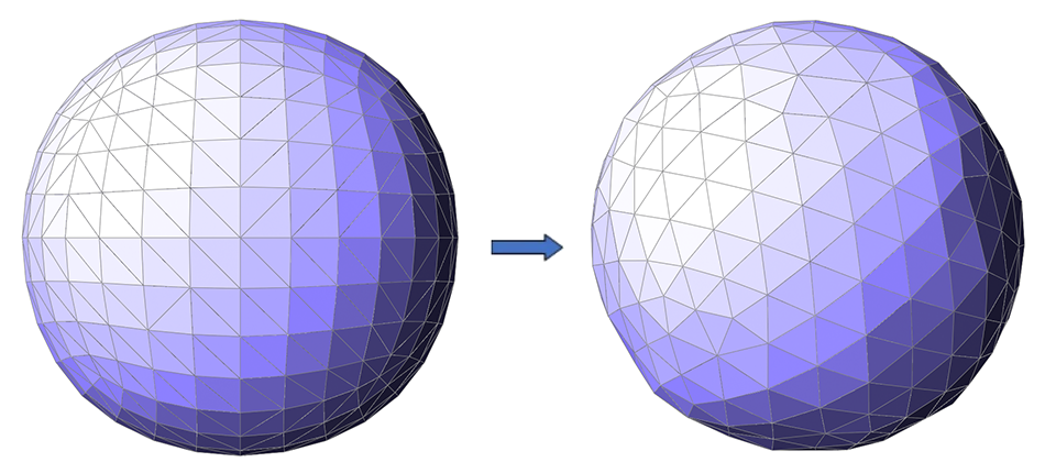
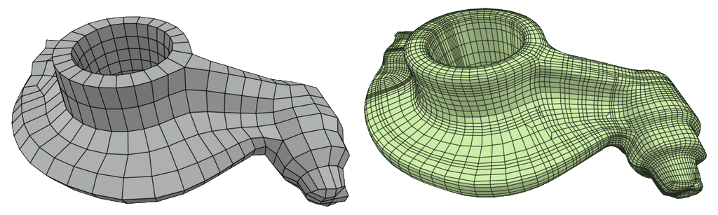
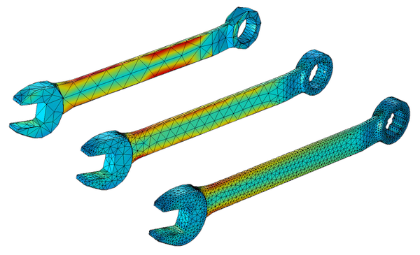
Figure 1: Different mesh resolutions for the same model.

Download PDF 

1. Why Refinement Matters

Refinement is the mechanism that determines where resolution is allocated within a mesh. It transforms a coarse geometric approximation into a discretization capable of supporting accurate numerical simulation. While segmentation partitions geometry into meaningful regions, refinement controls the size, density, and alignment of elements within those regions.

In numerical simulation, the accuracy of a solution depends critically on the mesh. Let u denote the exact solution of a governing equation and u_h its discrete approximation on a mesh \mathcal{T}_\mathcal{h}. The discretization error satisfies:

\[u-uh≤C,hp\]

where h represents a characteristic element size and p the order of the numerical method. This relationship highlights a fundamental principle: reducing error requires reducing element size—but only where necessary.

Naïve refinement strategies that uniformly reduce h across the domain lead to excessive computational cost. Effective refinement instead seeks an optimal distribution of resolution.

In modern simulation workflows, refinement is essential for both accuracy and stability. Numerical solvers rely on well-resolved curvature, sharp features, boundary layers, and stress concentrations. When refinement is insufficient, simulations suffer from numerical noise, instability, and misleading results. When applied effectively, refinement produces meshes that are both computationally efficient and physically predictive.

At its core, refinement is not about increasing element count, but about placing resolution where it matters most.

This article presents the principles that govern mesh refinement, the criteria used to guide it, and the strategies employed in high-quality mesh generation.
2. Types of Refinement Strategies

Refinement strategies can be categorized based on how they distribute resolution across the domain. Each approach addresses a different aspect of geometric or physical complexity.

2.1 Uniform Refinement

Uniform refinement subdivides all elements equally across the mesh.

\[h\left(x\right)=h_0\] for all x in the domain.

Its primary advantages are simplicity, predictability, and ease of implementation, making it useful for debugging and baseline comparisons.

However, uniform refinement is inherently inefficient. Most geometries contain localized features that require higher resolution, while large regions remain smooth and over-resolved. As a result, uniform refinement significantly increases computational cost without proportionally improving accuracy.

Uniform Refinement

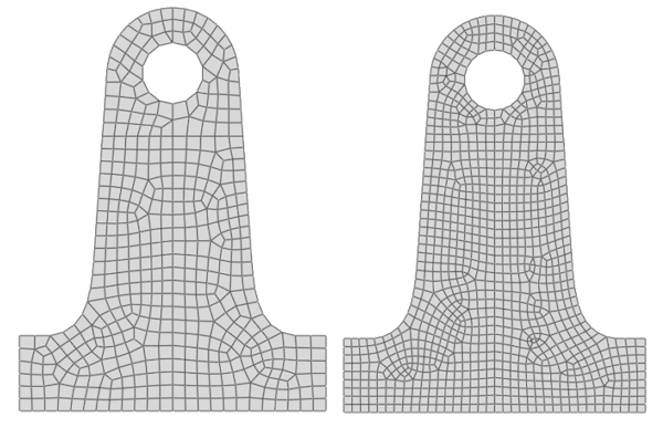
Figure 2: Uniform refinement example.

2.2 Adaptive Refinement

Adaptive refinement allocates resolution selectively, guided by geometric or numerical indicators. Instead of uniformly increasing element density, it concentrates elements in regions of high error or complexity.

\[h\left(x\right)\rightarrow h_K {\ \ for\ each\ element\ }K\] based on an indicator \(\eta_K\). A common refinement criterion is:

\[\eta_K>\ \tau\] where \(\tau\) is a prescribed tolerance. Elements satisfying this condition are refined, concentrating resolution where it is most needed.

This approach dramatically improves efficiency but introduces additional challenges. Care must be taken to maintain element quality, avoid excessive distortion, and ensure smooth transitions between refined and coarse regions.

Adaptive Refinement

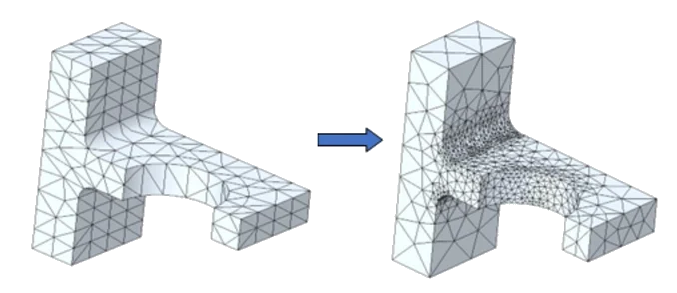
Figure 3: Adaptive refinement example.

2.3 Feature-Aligned Refinement

Engineering geometries often contain sharp edges, ridges, and creases that define their structural and functional behavior. Feature-aligned refinement ensures that mesh elements conform to these features rather than smoothing or approximating them.

Let \(\Gamma_f\) denote a set of feature curves (e.g., sharp edges). Feature-aligned refinement enforces:

\[h\left(x\right)\ll h_0{\ \ for\ }x\in\Gamma_f\]

and constrains element orientation to align with the tangent direction of the feature. This preserves geometric discontinuities and improves numerical accuracy near sharp gradients.

By aligning elements with feature lines, this strategy preserves geometric fidelity and improves numerical accuracy in regions where gradients are typically large or discontinuous.

Feature-Aligned Refinement

Figure 4: Feature-aligned refinement example.

2.4 Curvature-Driven Refinement

Curvature provides a natural indicator of geometric complexity. Regions of high curvature require smaller elements to maintain an accurate representation, while flatter areas can be discretized more coarsely.

Let \(\kappa\left(x\right)\) denote curvature magnitude. A common sizing relation is:

\[h\left(x\right)\propto\frac{1}{\sqrt{\left|\kappa\left(x\right)\right|+\epsilon}}\]

where \(\epsilon\) prevents singular behavior in flat regions.

Curvature-driven refinement adjusts element size according to curvature magnitude and variation, producing meshes that efficiently approximate smooth surfaces without unnecessary refinement in low-curvature regions.

Curvature-Driven Refinement

Figure 5: Curvature-driven refinement example.

2.5 Physics-Driven Refinement

In simulation-driven workflows, refinement is often guided by the solution itself. Physical quantities such as stress, vorticity, and heat flux reveal where additional resolution is required.

Let \(\eta_K\) be an a posteriori error estimator. The refinement process follows:

\[\mathcal{T}h\rightarrow\mathcal{T}h^\prime{\ \ such\ that\ \ }\eta_K\le\tau\]

for all elements.

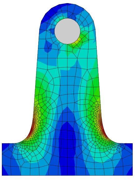
Physics-driven refinement typically operates in an iterative loop:

solve → estimate error → refine → solve again

This process, central to finite element and CFD methods, ensures that refinement is directly tied to simulation accuracy rather than purely geometric considerations.

Physics-Driven Refinement

Figure 6: Physics-driven refinement example.

3. Refinement Criteria

Refinement decisions are driven by indicators that measure geometric, topological, or numerical complexity. These criteria collectively define how resolution is distributed across the domain.

Importantly, they can be interpreted as defining a spatial sizing field ( h\left(x\right) ), which prescribes the desired element size throughout the mesh.

3.1 Geometric Criteria

Geometric criteria rely solely on the shape of the domain and include:

  • Principal curvatures \( k_1,k_2 \)
  • Curvature gradients \( \nabla k \)
  • Distance to features \( d\left(x,\Gamma_f\right) \)
  • Local thickness measures

These indicators ensure that the mesh accurately represents the underlying geometry, independent of any simulation results.

3.2 Topological Criteria

Topology influences how refinement must be applied to preserve mesh validity and structure.

Let \(v\) denote a vertex with valence \(d\left(v\right)\). Regions where:

\[d\left(v\right)\gg\bar{d}\]

where \(\bar{d}\) is average valence may require refinement to maintain regularity.

Additional indicators include:

  • Junctions and branching points
  • Regions sensitive to projection or parameterization
  • Segmentation boundaries

Such areas often require additional resolution to prevent degeneracies and maintain consistency across the mesh.

3.3 Numerical Criteria

Numerical criteria are derived from the solution field and drive refinement toward improved simulation accuracy.

A common approach uses residual-based estimators:

\[\eta_K=R_K+\sum_{e\subset\partial K}J_e\]

where \(R_K\) is the element residual and \(J_e\) represents flux jumps across element interfaces.

More advanced methods use the Hessian \(H\left(u\right)\) of the solution to guide anisotropic refinement.

Common indicators include:

  • A posteriori error estimators
  • Residual-based measures
  • Gradient discontinuities between elements
  • Hessian-based anisotropy indicators

These criteria ensure that the mesh adapts not only to geometry, but also to the underlying physics.

4. Refinement Patterns

Refinement is defined not only by where it is applied, but also by how elements are modified.

4.1 Isotropic Refinement

Isotropic refinement reduces element size uniformly in all directions. It is simple and robust, making it well-suited for general-purpose refinement and curvature-based adaptation. Isotropic refinement enforces:

\[h_x=h_y=h_z\]

producing elements with uniform scaling in all directions.

However, isotropic refinement becomes inefficient in problems with strong directional behavior, where resolution is only needed along specific directions. This is effective for general-purpose refinement but inefficient in anisotropic solution fields.

Isotropic Refinement

Figure 7: Isotropic refinement example.

4.2 Anisotropic Refinement

Anisotropic refinement adjusts both the size and shape of elements, stretching them along preferred directions. This enables accurate resolution with significantly fewer elements compared to isotropic approaches.

It is particularly important in:

  • Boundary layers in CFD
  • Thin shells and plates
  • Flow-aligned structures
  • Regions with highly directional gradients

Let \(H\left(u\right)\) denote the Hessian of the solution. Its eigen-decomposition:

\[H=Q\Lambda Q^T\]

defines principal directions and curvature magnitudes. Element stretching is aligned with eigenvectors, with sizes inversely proportional to eigenvalues. Anisotropic refinement is typically guided by eigen-analysis of the Hessian or a metric tensor, which determines element orientation and aspect ratio.

This enables accurate approximation with significantly fewer elements.

Anisotropic Refinement

Figure 8: Anisotropic refinement example.

4.3 Metric-Based Refinement

Metric-based refinement provides a unifying framework for modern mesh adaptation. It defines a Riemannian metric field over the domain, prescribing desired element size, shape, and orientation at every point.

A symmetric positive-definite tensor field M\left(x\right) defines the desired element geometry:

\[|| \mathbf{e} ||_M^2 = \mathbf{e}^T M(x) \mathbf{e}\]

The mesh is constructed such that elements are approximately unit-sized in the metric space:

\[e^T M(x) e \approx 1\]

The mesh is then generated to be uniform in this metric space.

This approach enables:

  • Smooth transitions between refinement levels
  • Precise directional control
  • Integration of geometric and numerical criteria
  • Consistent error-driven adaptation

This framework naturally incorporates anisotropy, smooth grading, and multiple refinement criteria.

Metric Based Refinement: From Theory to Engineering Practice
Read more 

5. Refinement Pipelines

In practice, refinement operates within broader workflows that connect geometry processing, meshing, and simulation. These pipelines differ in what drives refinement decisions.

5.1 Geometry-First Pipeline

The geometry-first pipeline begins with segmentation and geometric analysis. Curvature and features are identified, followed by initial mesh generation and subsequent refinement based on geometric criteria.

This approach is commonly used in CAD-based workflows, where geometric fidelity is the primary concern.

5.2 Simulation-Driven Pipeline

In simulation-driven workflows, refinement is guided by numerical error. A coarse mesh is first generated and used to compute an approximate solution \(u_h\). Error estimates \(\eta_K\) then identify regions requiring refinement, and the process is repeated iteratively.

\[\max_K \eta_K \le \tau\]

This pipeline is essential in applications where accuracy of the solution is the dominant objective.

5.3 Hybrid Pipeline

Hybrid approaches combine geometric and numerical refinement. Geometry ensures accurate representation of shape, while simulation data ensures physical accuracy:

\[M\left(x\right)=M_{\mathrm{geom}}\left(x\right)+M_{\mathrm{phys}}\left(x\right)\]

ensuring both geometric fidelity and solution accuracy.

This combination is particularly effective in complex engineering problems, where both geometry and physics play critical roles.

6. Refinement and Mesh Quality

Refinement must preserve element quality to be effective. Poor refinement can introduce:

Quality constraints can be expressed as:

\[\frac{h_{max}}{h_{min}}\le C\]

For neighboring elements, ensuring smooth grading.

Maintaining mesh validity requires continuous monitoring of aspect ratios, angles, and element distortion.

Refinement and mesh quality are fundamentally interconnected; increasing resolution without maintaining quality can negate any potential accuracy gains.

7. Refinement in Real Engineering Workflows

Refinement theory becomes meaningful only when it is applied to real geometries, real physics, and real constraints.

The following case studies illustrate how geometric, metric based, and error driven refinement strategies translate into practical meshing decisions across different engineering domains.

Each example highlights a distinct refinement signal — curvature, flow direction, or stress gradients — and shows how the mesh adapts to capture the underlying behavior.

7.1 High Curvature Mechanical Part

Curvature Driven + Feature Aligned Refinement

Mechanical components often contain a mixture of smooth blends and sharp geometric features: fillets, chamfers, holes, ribs, and transitions between functional surfaces. These regions are precisely where geometric complexity is highest and where solvers are most sensitive to under resolution.

Geometric Signals

Curvature-driven sizing ensures:

\[h\left(x\right)\sim\frac{1}{\sqrt{\kappa\left(x\right)}}\]

capturing small radii and smooth transitions accurately. The result is a mesh that accurately captures both smooth transitions and distinct geometric features.

  • Principal curvature spikes along fillets and blends.
  • Curvature gradients increase near transitions between flat and curved regions.
  • Feature lines (sharp edges, hole boundaries) introduce geometric discontinuities.

Refinement Behavior

Curvature driven refinement reduces element size in regions where curvature magnitude is high, ensuring that small radii are represented with sufficient fidelity. Feature aligned refinement then reinforces this by concentrating resolution along edges and hole perimeters, preventing geometric smoothing or loss of sharpness.

Engineering Impact

  • Accurate stress prediction around fillets and holes.
  • Improved convergence in structural solvers.
  • Preservation of functional geometry (e.g., sealing surfaces, load paths).
  • Reduced global element count compared to uniform refinement.

This case demonstrates how purely geometric signals can guide refinement to produce meshes that respect both shape and mechanical behavior.

7.2 CFD Boundary Layer

Anisotropic + Metric Based Refinement

Fluid dynamics introduces a fundamentally different challenge: the physics itself is highly directional. Boundary layers form thin regions near walls where velocity gradients are steep in the normal direction but smooth tangentially. Capturing this behavior requires elements that are extremely stretched along the flow direction.

Physical Signals

  • Velocity gradient tensor identifies the direction of steepest change.
  • Vorticity magnitude highlights shear layers.
  • Wall normal gradients define boundary layer thickness.

Refinement Behavior

Anisotropic refinement produces long, thin elements aligned with the flow direction. The Riemannian metric tensor encodes this anisotropy:

  • Small metric eigenvalues in the wall normal direction → very fine spacing.
  • Large eigenvalues tangentially → elongated elements.

Metric based refinement ensures that these anisotropic elements transition smoothly into the isotropic far field mesh, avoiding abrupt jumps in element size that would destabilize the solver.

Engineering Impact

  • Accurate resolution of shear layers and near wall behavior.
  • Stable convergence in Navier-Stokes solvers.
  • Reduced computational cost compared to isotropic refinement.
  • Ability to capture flow separation, recirculation, and vortex shedding.

This case shows how physics driven anisotropy is essential for CFD accuracy and efficiency.

7.3 Adaptive Stress Analysis

Error Driven Iterative Refinement

In structural analysis, the true stress distribution is often unknown until the simulation is performed. Regions of high stress concentration — near notches, load application points, or material transitions — may not be obvious from geometry alone.

Numerical Signals

  • A posteriori error estimators quantify local discretization error.
  • Stress gradient jumps across elements reveal under resolved regions.
  • Hessian based indicators identify curvature in the stress field.

Refinement Behavior

The workflow follows an iterative loop:

  1. Generate a coarse mesh.
  2. Solve the structural problem.
  3. Compute error indicators.
  4. Refine locally where error is high.
  5. Re solve and repeat until convergence.

Refinement concentrates around stress concentrations, crack tips, fillet roots, and load introduction points. The rest of the domain remains coarse, minimizing computational cost.

Engineering Impact

  • Accurate prediction of peak stresses and failure locations.
  • Reliable fatigue and durability assessments.
  • Efficient use of computational resources.
  • Convergence toward the true stress field without global refinement.

This case illustrates how numerical feedback drives refinement when geometric intuition is insufficient.

8. Coclusion

Mesh refinement is a fundamental component of high-quality mesh generation, governing how resolution is distributed across geometry and simulation domains. Effective refinement strategies rely on geometric, topological, and numerical criteria, and employ isotropic or anisotropic patterns as required.

Modern refinement strategies increasingly rely on metric-based formulations, enabling unified treatment of isotropic and anisotropic adaptation, smooth grading, and error control.

Ultimately, high-quality meshes are not the result of uniformly increasing resolution, but of intelligent, targeted refinement that strategically distributes it according to the underlying structure of the problem, balancing accuracy, efficiency, and stability.