Mesh Quality Metrics Every Engineer Should Know

Why Mesh Quality Matters

A mesh is more than just a collection of elements - it's the foundation of simulation accuracy, stability, and efficiency, in other words it is the numerical backbone of the simulation. Poor mesh quality leads to distorted gradients, destabilized solvers, and wasted time. Good mesh quality enables reliable simulations, faster convergence and reduces the need for brute-force refinement.
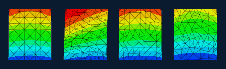
good_bad_mesh

Figure 1: Different mesh qualities for the same region.

This article breaks down the most important metrics engineers should understand, visualize, and apply, with detailed explanations and illustrative examples to deepen your understanding.
Core Metrics

Aspect Ratio

What is Aspect Ratio?
Aspect Ratio

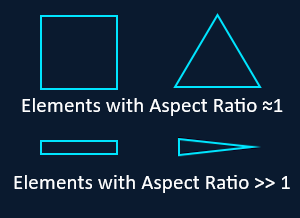
Aspect ratio measures how stretched or elongated a mesh element is compared to its ideal shape.

  • For triangles, the ideal shape is equilateral.
  • For quadrilaterals, it is a square.
  • For hexahedra, it is a cube.

Formula (simplified):

  • For quads or hexes:  \( Aspect\ Ratio = LongestEdgeLength / ShortestEdgeLength \)
  • For triangles:  \( Aspect\ Ratio = LongestEdge / HeightFromOppositeVertex \)
Accepted Values of Aspect Ratio based on element type

Aspect ratio values vary based on the type of element and the specific application, but general guidelines are:

  • Triangles:  Ideal aspect ratio is 1 (equilateral), values up to 3 are often acceptable, but above 5 can lead to poor results.
  • Quadrilaterals:  Ideal aspect ratio is 1 (square), values up to 5 may be acceptable, but above 10 can cause issues.
  • Hexahedra:  Ideal aspect ratio is 1 (cube), values up to 5 may be acceptable, but above 10 can lead to significant problems.
Why it matters

High aspect ratio elements can:

  • Distort gradients:  Especially in regions with rapid physical changes.
  • Cause solver instability:  Poor conditioning of the stiffness matrix.
  • Reduce accuracy:  Especially in interpolation and integration.
  • Slow convergence:  Solvers may need more iterations or fail entirely.

In boundary layers (e.g. CFD), high AR is sometimes intentional — but only when aligned with the flow and handled by specialized solvers.

Aspect ratio is directional: A long thin element aligned with the flow may be fine; misaligned, it is trouble.

Skewness

What is Skewness?

Skewness measures how much a mesh element deviates from its ideal angular shape.

  • For triangles, the ideal shape is equilateral (all angles 60°).
  • For quadrilaterals, it is a square (all angles 90°).
  • For hexahedra, it is a cube.

Skewness increases when angles become too small or too large — distorting interpolation and gradient calculations.

Skewness
How is it calculated?

For equilateral shapes, skewness is defined as:

\[ Skewness=\ \frac{optimal\ Cell\ Size-Cell\ Size}{Optimal\ Cell\ Size} \]

where the optimal cell size is the size of the equilateral cell with the same circumradius.

For equiangular shapes we have:

\[ Skewness=\ max\left[\frac{\theta_{max}-\theta_e}{180-\theta_e},\ \frac{\theta_e-\theta_{min}}{\theta_e}\right]] \]

where:

  • \(θ_{max}\) : largest angle in the face
  • \(θ_{min}\) : smallest angle in the face
  • \(θ_e\) : angle for an equiangular face (60 for triangle, 90 for square)
Allowed values for Skewness

Skewness values range from 0 (perfectly equilateral) to 1 (completely degenerate). General guidelines are:

  • Skewness < 0.25:  Good quality.
  • Skewness 0.25 - 0.5:  Acceptable, but may cause issues in sensitive regions.
  • Skewness 0.5 - 0.75:  Poor quality, likely to cause solver instability and inaccurate results.
  • Skewness > 0.75:  Very poor quality, almost certainly causing solver instability and inaccurate results.
Why it matters

High skewness can:

  • Distort gradients — especially in CFD and FEA
  • Cause convergence issues — solvers may oscillate or diverge
  • Reduce accuracy — especially in second-order schemes

Skewness is especially critical in finite volume methods, where face interpolation depends on geometric alignment.

Key points
  • Skewness is independent of size — a tiny triangle can be perfectly shaped.
  • It interacts with aspect ratio and orthogonality — high AR often increases skewness.
  • Some solvers tolerate moderate skewness if interpolation schemes are robust (e.g. upwind vs central differencing)

Jacobian Determinant

The Jacobian determinant is one of the most critical mesh quality metrics, especially in finite element analysis (FEA) and computational fluid dynamics (CFD). It tells you whether your mesh elements are valid, well-shaped, and numerically stable.

The Jacobian is not just a shape metric — it’s a mapping metric. Even a visually decent element can have a bad Jacobian if its internal mapping is distorted.

What is Jacobian Determinant?

In mesh terms, the Jacobian determinant measures how well an element maps from its reference shape (ideal element in parametric space) to its actual shape in physical space.

  • Reference element: A perfect square, triangle, or hexahedron in a normalized coordinate system.
  • Physical element: The actual shape in your mesh, possibly distorted.

The Jacobian matrix contains partial derivatives of this transformation. Its determinant tells you how much the element is stretched, compressed, or flipped.

The meaning of the Jacobian Determinant
Jacobian ValueMeaningAction
>0.1 and <10Valid and well-shapedAcceptable
≈ 1Ideal mappingExcellent
≈ 0Collapsed elementMust fix
< 0Inverted elementFatal error
  • Measures the quality of the transformation from the reference (ideal) element to the actual physical element.
  • Positive values mean the element is valid.
  • Near-zero or negative values mean the element is degenerate or flipped — which breaks the simulation.
  • Ideal values are positive and close to 1, indicating a valid and well-shaped element.

Smoothness

Smoothness is one of the most underrated mesh quality metrics — but it plays a huge role in solver stability, gradient accuracy, and adaptive refinement.

Smoothness measures how gradually element size and shape change across the mesh.

It is also called expansion rate, growth factor, or uniformity.

Definition
\[ Smoothness = \max\left(\frac{Size_{Element\ i+1}}{Size_{Element\ i}}, \frac{Size_{Element\ i}}{Size_{Element\ i+1}}\right) \]
  • A ratio close to 1 means smooth transitions.
  • A ratio significantly greater than 1 indicates abrupt changes in element size.

Smoothness is crucial for maintaining solver stability and ensuring accurate gradient calculations.

What is a good smoothness profile?
Smoothness Ratio Quality Description
1.0 - 1.2ExcellentGradual change
1.2 - 1.5AcceptableMild transition
1.5 - 2.0PoorAbrupt jump
> 2.0ProblematicSolver may diverge
Why it matters

Poor smoothness can:

  • Disrupt convergence — solvers struggle with abrupt changes in stiffness
  • Cause numerical diffusion — gradients get smeared across large jumps
  • Mask other issues — bad Jacobians or skewness may hide in uneven regions
  • Break adaptivity — refinement algorithms rely on smooth transitions

Smoothness is especially critical in boundary layers, shock regions, and multi-scale simulations.

Key points

Smoothness is not about shape, but about size transitions.

  • It’s often violated near interfaces, boundaries, or refined regions.
  • Some solvers apply smoothing algorithms to fix it — Laplacian smoothing, optimization-based smoothing, or deep learning methods.

Orthogonality

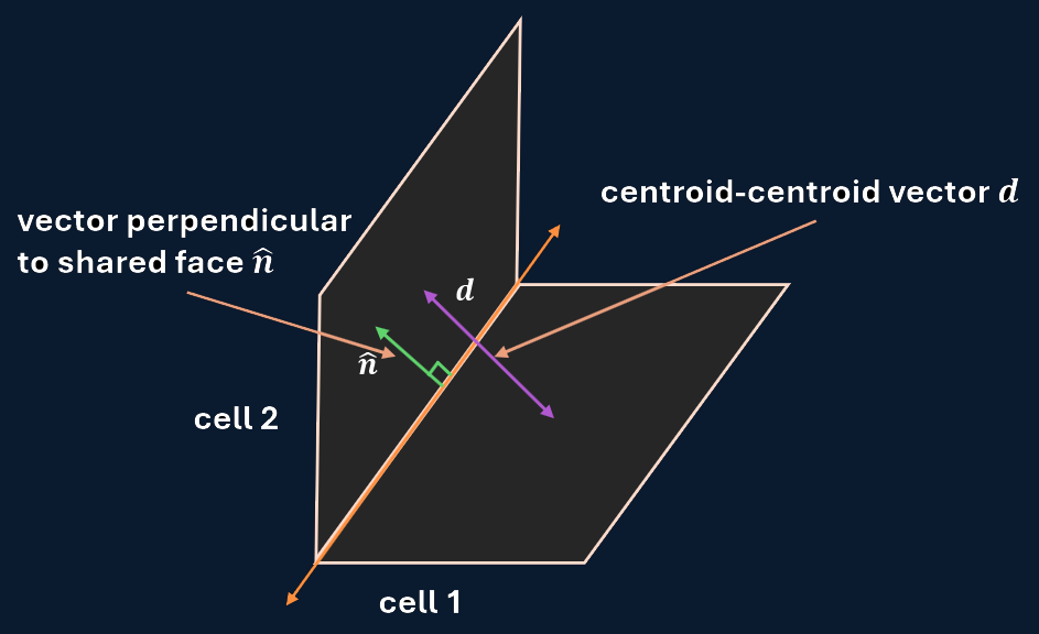
Orthogonality is a subtle but powerful mesh quality metric — especially in finite volume and finite difference methods, where fluxes and gradients are computed across element faces

What is Orthogonality?

Orthogonality measures how well the faces of 3D mesh elements align with the flow direction or gradient direction. It is especially important in CFD and FEA, where accurate flux calculations depend on face alignment.

Orthogonality is often measured as the angle between the face normal and the vector connecting the centroids of adjacent elements. A perfectly orthogonal face has an angle of 0°.

Orthogonality measures the angle between:

  • The face normal vector of a mesh element and
  • The vector connecting adjacent cell centers (or the direction of flow / gradient)

Ideal case:

  • Face normal ⟂ cell-center vector → angle ≈ 90°

Poor case:

  • Face normal tilted → angle far from 90°
Orthogonality
What is a good Orthogonality value?
Orthogonality AngleQualityDescription
85° - 90°ExcellentNear perfect alignment
70° - 85°AcceptableMinor misalignment
50° - 70°PoorLikely to cause flux errors
< 50°ProblematicPossible Solver instability

Some solvers use a normalized orthogonality metric (0 = perfect, 1 = worst), but angle-based interpretation is more intuitive.

Why it matters

Poor orthogonality can:

  • Distort flux calculations — especially in CFD, where face normals are critical for accurate fluxes.
  • Cause convergence issues — solvers may struggle with non-orthogonal faces.
  • Break pressure-velocity coupling in compressible flows
  • Reduce accuracy — especially in second-order schemes that rely on face alignment.

Orthogonality is especially critical in CFD, heat transfer, electromagnetics, boundary layers, shock regions, and multi-scale simulations.

Key Points
  • Orthogonality is directional — it depends on the physics being simulated.
  • It interacts with skewness — highly skewed elements often have poor orthogonality.
  • Structured meshes (e.g. Cartesian grids) have excellent orthogonality by design.
  • Unstructured meshes need careful alignment or correction.