Differential Geometry for CAE: A Practical Introduction

Geometric Quantities, Discrete Operators, and Their Role in Simulation Workflows

This article examines differential geometry as a mathematical and computational foundation for modern Computer Aided Engineering. It concentrates on the geometric quantities most relevant to analysis and implementation—tangent vectors, surface normals, metric tensors, curvature measures, and their discrete analogues on triangulated and quadrilateral meshes—and on the ways these quantities enter meshing, shell formulations, contact formulations, surface operators, post-processing, and shape optimization. The aim is to establish a concise technical framework that links geometric representation to numerical treatment and, in turn, to engineering outcomes, with particular emphasis on model fidelity, formulation consistency, and solver robustness.

Download PDF 

1. Relevance of Differential Geometry to Computer Aided Engineering

In Computer Aided Engineering, geometry is not merely a passive representation of form; it actively shapes simulation quality, numerical stability, and engineering judgment.

Whether the objective is meshing, contact resolution, shell analysis, or shape optimization, reliable computation depends on the ability to quantify how a surface bends, stretches, and changes orientation.

Differential geometry provides the mathematical and computational foundation for:

For most engineering teams, the priority is not theoretical completeness but operational relevance.

In CAE, the value of differential geometry lies in its computational subset: the concepts that directly influence model fidelity, element behavior, solver robustness, and downstream interpretation.

This article isolates that practical core and relates it directly to the CAE workflow.

2. Surface Representation as a Parametric Mapping

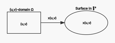
A productive way to represent a surface is as a mapping:

\[{x}\left(u,v\right):\Omega\subset{R}^{2}\rightarrow{R}^{3}\]

This formulation encompasses:

From this representation, tangent vectors, surface normals, and curvature follow naturally. The next step is to examine the local differential quantities that make this representation computationally useful.
(u,v)-domain Ω (u,v) Surface in ℝ³ x(u,v) x(u,v)

Figure 1: Parametric Surface.

3. Tangent Fields and the First Fundamental Form

3.1 Tangent Vectors and the Tangent Plane

\[{x}_{u}=\frac{\partial{x}}{\partial u}, {x}_{v}=\frac{\partial{x}}{\partial v}\]

Together, these vectors define the tangent plane at the point of interest.

Surface in ℝ³ x(u,v) \(x_u\) \(x_v\)

Figure 2: Tangent Vectors on a Surface.

3.2 The First Fundamental Form and Metric Tensor

The first fundamental form encodes the inner products of tangent vectors:

\[E = x_u \cdot x_u, F = x_u \cdot x_v, G = x_v \cdot x_v\]

It determines how distances and angles are measured locally on the surface. Once that local metric structure is established, the analysis can turn from measurement to bending.

In CAE, the metric tensor is central to:

  • element distortion
  • surface Jacobians
  • evaluation of shell membrane strains
  • mapping of integration points

1. Computing the Metric Tensor (C++)

template <typename T>
struct SurfacePoint
{
    basepoint3<T> x; // position
    basevec3<T> xu;  // ∂x/∂u
    basevec3<T> xv;  // ∂x/∂v
    basevec3<T> n;   // unit normal
};

template <typename T>
struct MetricTensor
{
    T E, F, G;
};
template <typename T>
inline MetricTensor<T> computeMetric(const SurfacePoint<T> &p)
{
    MetricTensor<T> m;
    m.E = dot(p.xu, p.xu);
    m.F = dot(p.xu, p.xv);
    m.G = dot(p.xv, p.xv);
    return m;
}

4. Surface Normals and Curvature Measures

4.1 Surface Normal Definition and Use

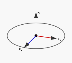
The surface normal is defined as the cross product of the tangent vectors, normalized to unit length:

\[ {n}=\frac{{x}_{u}\times{x}_{v}} {\parallel{x}_{u}\times{x}_{v}\parallel} \]

Applications include:

  • contact formulations
  • shell formulations
  • boundary-condition specification
  • CAD-to-mesh consistency
xᵤ xᵥ n

Figure 3: Surface Normal Vector.

4.2 Curvature Measures and Differential Characterization

Curvature quantifies local surface bending.

Its evaluation, in turn, requires second derivatives:

\[ {x}_{uu},\ {x}_{uv},\ {x}_{vv} \]

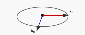
These terms define the shape operator, from which we obtain the principal curvature measures used in analysis. In practice, however, CAE workflows usually require discrete approximations of these continuous quantities.

  • principal curvatures \(k_1,k_2\)
  • principal directions
  • mean curvature \(H\)
  • Gaussian curvature \(K\)
k₁ k₂

Figure 4: Principal Curvatures and Directions

1. Computing the Metric Tensor (C++)

template <typename T>
struct CurvatureTensor
{
    T k1, k2;
    basevec3<T> d1, d2; // principal directions
};

template <typename T>
CurvatureTensor<T> computeCurvature(
    const SurfacePoint<T>& p,
    const basevec3<T>& xuu,
    const basevec3<T>& xuv,
    const basevec3<T>& xvv)
{
    // Build first and second fundamental forms
    T E = dot(p.xu, p.xu);
    T F = dot(p.xu, p.xv);
    T G = dot(p.xv, p.xv);

    T L = dot(xuu, p.n);
    T M = dot(xuv, p.n);
    T N = dot(xvv, p.n);
    // Solve generalized eigenproblem |II - k I| = 0
    // (implementation omitted for brevity)

    CurvatureTensor<T> K;
    // fill K.k1, K.k2, K.d1, K.d2
    return K;
}

5. Discrete Differential Geometry on Computational Meshes

Most CAE workflows operate on triangulated or quadrilateral meshes.

As a result, smooth geometric quantities must be approximated in discrete form.

5.1 Discrete Normal Construction

Common discrete normal definitions include:

  • face normals
  • area-weighted vertex normals
  • angle-weighted vertex normals

3. Angle-Weighted Vertex Normal (C++)

template <typename T>
basevec3<T> computeVertexNormal(int v, const Mesh<T>& mesh) {
    basevec3<T> n(0.0);
    for (auto f : mesh.facesAroundVertex(v)) {
        basevec3<T> fn = mesh.faceNormal(f);
        T angle = mesh.cornerAngle(f, v);
        n += angle * fn;
    }
    return normalize(n);
}

5.2 Discrete Curvature Estimation

Widely used discrete curvature estimators include:

  • Meyer et al. mean curvature estimator
  • normal variation
  • quadric error metrics
  • umbrella operators

Figure 5: Discrete Curvature Neighbohood.

5.3 The Discrete Laplace–Beltrami Operator

Discrete surface operators, such as the Laplace–Beltrami operator, are essential for smoothing, parameterization, and curvature flow.

\[ \Delta \mathbf{x} = \sum_{j} w_{ij} \left( \mathbf{x}_j - \mathbf{x}_i \right) \]

This operator is used for:

  • smoothing
  • curvature flow
  • parameterization
  • shape optimization

Taken together, these discrete operators translate differential geometry into forms that can be applied directly within engineering workflows. The next section considers where those quantities enter the CAE process in practice.

Example 4. Cotangent Laplacian (C++)

template <typename T>
inline basevec3<T> laplacian(int v, const Mesh<T> &mesh)
{
    basevec3<T> sum(0.0f);
    T wsum = 0.0;

    for (auto e : mesh.edgesAroundVertex(v))
    {
        int j = mesh.otherVertex(e, v);
        T w = cotangentWeight(mesh, v, j);
        sum += w * (mesh.position(j) - mesh.position(v));
        wsum += w;
    }

    return (wsum > 0.0) ? sum / wsum : basevec3<T>(0.0f);
}

6. Role of Differential Geometry in the CAE Workflow

The geometric quantities and discrete operators described above are not just mathematical abstractions; they are integral to the CAE workflow at multiple stages.

6.1 From CAD to Mesh Generation

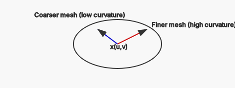
During meshing, the metric tensor and curvature measures guide element sizing and distribution. High curvature regions require finer meshes to capture geometric fidelity, while flatter areas can be meshed more coarsely. Surface normals ensure that the mesh conforms to the intended geometry, particularly for shell elements.

Other mesh generation decisions, such as the choice of element type (triangular vs. quadrilateral) and the handling of sharp features, also depend on geometric analysis.

x(u,v) Finer mesh (high curvature) Coarser mesh (low curvature)

Figure 6: Curvature-Driven Refinement.

6.2 From Mesh Representation to Solver Formulation

In solver preparation, these differential quantities are used to:

  • compute surface Jacobians
  • construct local frames
  • evaluate shell bending and membrane strains
  • ensure consistent normals for contact

In shell formulations, the metric tensor and curvature measures directly influence the stiffness matrix and the evaluation of membrane and bending strains.

In contact mechanics, surface normals are essential for defining contact constraints and ensuring accurate force transmission.

In shape optimization, curvature-based regularization can help maintain smoothness and prevent mesh degeneration.

In post-processing, curvature measures can be used to identify critical regions, such as stress concentrations or areas of high deformation, and to guide visualization strategies.

6.3 From Solver Output to Post-Processing Interpretation

After the solver has produced results, the geometric quantities can be used for:

  • stress-field visualization on curved surfaces
  • alignment between principal stress directions and principal curvature directions
  • curvature-based filtering of noisy fields

These applications show that differential geometry is not confined to isolated algorithms; it spans the full simulation pipeline. That breadth, in turn, motivates a coherent implementation strategy.

7. Concluding Remarks

Taken as a whole, the preceding sections show that differential geometry is not a peripheral mathematical topic in CAE; it is part of the discipline’s operational foundation.

It provides the language and structure needed to connect geometric representation to numerical treatment and, ultimately, to engineering outcomes. In practical terms, it clarifies:

For TheMeshProject, the strategic implication is clear: differential geometry should be treated not as background theory, but as core engineering infrastructure linking geometric representation, numerical treatment, and practical simulation outcomes.